
The edge is a battlefield of constraints: latency, power, and dumb hardware
Why edge ML isn't an optimization problem, but a systems engineering one

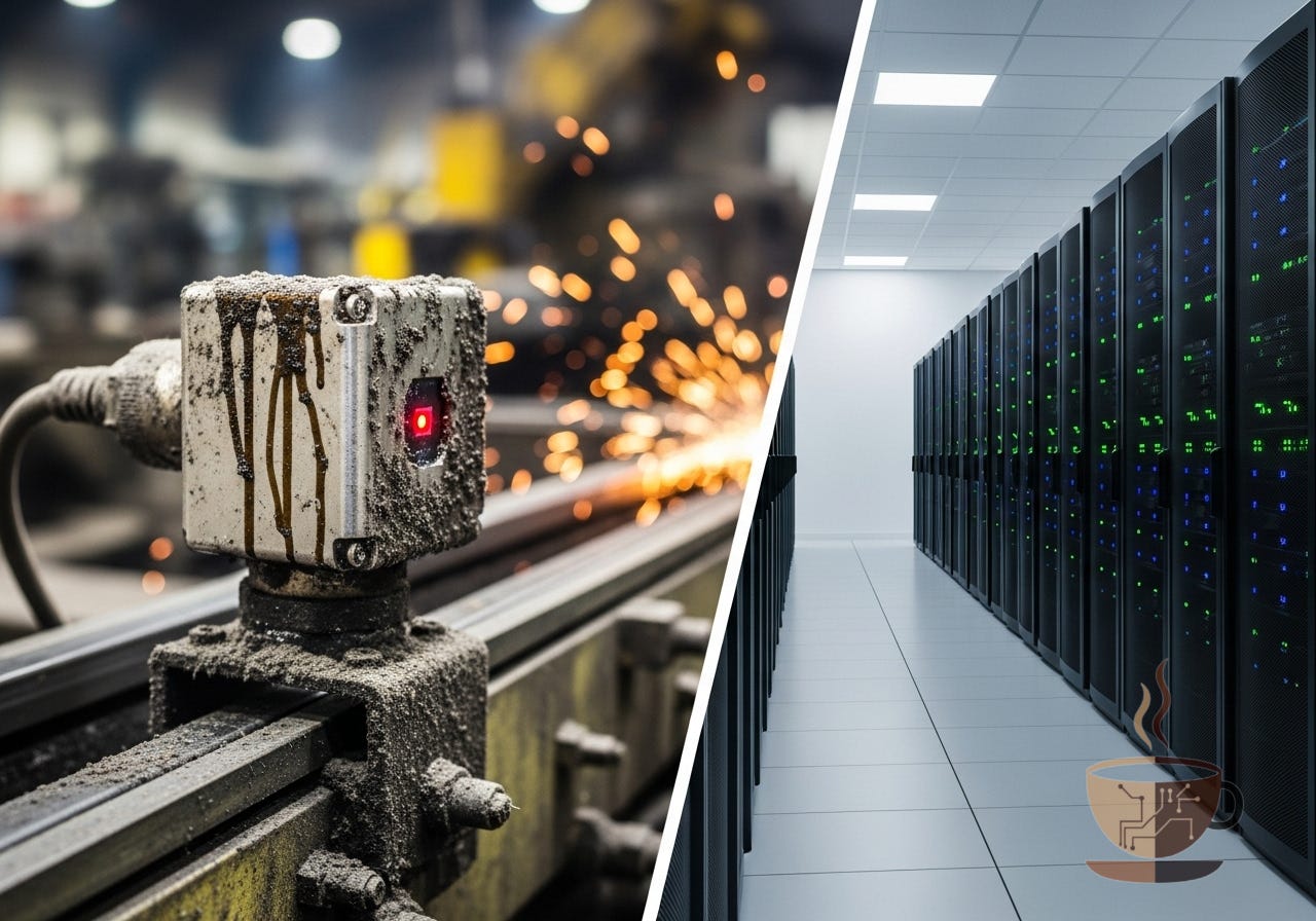
The cloud is a data center. It’s a clean room with climate control, redundant power supplies, and racks of servers that can be provisioned on demand. When you need more compute, you spin up another instance. When you need more memory, you choose a bigger machine type. The infrastructure abstracts away the physical world, giving you the comfortable illusion of infinite resources.
The edge is a muddy trench.
It’s a camera mounted on a factory floor where the ambient temperature swings 40 degrees and vibrations from heavy machinery shake loose your assumptions about stable sensor readings. It’s a battery-powered device strapped to a wind turbine, lashed by rain and isolated from any network connection for days at a time. It’s a sensor in a delivery vehicle bouncing over potholes, losing GPS signal in tunnels, and running on a power budget measured in milliwatt-hours.
The prevailing narrative in machine learning circles is seductive and incomplete: “Running ML on the edge is about model optimization.” Compress your neural network. Prune some weights. Quantize to INT8. Deploy. This framing treats edge deployment as a tail-end optimization problem, a final polish you apply to a model that was designed in the comfortable abstractions of a Jupyter notebook.
This is dangerously wrong. It’s like saying winning a battle is just about having a sharp spear.
Successful edge deployment is not an ML problem solved with optimization; it is a systems engineering problem solved by designing for a hostile environment. Your primary goal is not peak accuracy on a holdout set. It’s operational resilience in conditions that will actively try to kill your system.
Part 1: the four horsemen of the edge apocalypse
These aren’t challenges you can engineer around with clever tricks. They are non-negotiable laws of physics. You don’t negotiate with them.
1. Latency
When people talk about edge inference latency, they fixate on one number: model inference time. “Our network runs in 15ms!” This is a dangerous simplification.
Your latency budget encompasses the entire photon-to-insight pipeline:
t_total = t_capture + t_pre + t_infer + t_postt_capture: sensor acquisition time. How long does it take to grab a frame from the camera, read from the accelerometer, or digitize an analog signal?
t_pre: pre-processing. Resizing images, normalizing inputs, converting color spaces. On weak hardware, this can dominate your budget.
t_infer: the model’s forward pass. This is the only part most people measure.
t_post: post-processing. Non-maximum suppression for object detection, Kalman filtering for tracking, formatting outputs for downstream systems.
In industrial robotics, a 20-millisecond delay between sensor input and actuator response is a system failure. The robot arm misses its target. The part goes into the reject bin. In autonomous navigation, that same delay is a disaster. The vehicle doesn’t see the obstacle in time. Physics doesn’t care about your model’s F1 score.
The latency budget is the ultimate arbiter of your system’s design. It dictates:
Which model architecture you can use (transformers with quadratic attention? Probably not.)
Which hardware you can target (a Raspberry Pi? Maybe. A microcontroller? Definitely constraints.)
How you structure your data pipeline (can you afford to batch inputs, or must you process them one at a time?)
2. Power
Every operation costs energy. A CPU cycle. A memory access. A floating-point multiplication. These costs accumulate, and on a battery-powered device, they add up to a finite number of joules—your device’s lifespan.
The Joule budget is as real as your bank account. Spend too fast, and you’re dead.
Consider the power profile of a typical edge device:
Idle state: 10-50mW (microcontroller sleeping, sensors off)
Active sensing: 200-500mW (camera on, preprocessing running)
Inference: 1-5W (neural network accelerator fully engaged)
Radio transmission: 500mW-2W (Wi-Fi or cellular upload)
A simple calculation: A device with a 10Wh battery running continuous inference at 2W has a battery life of 5 hours. If your application requires 24-hour operation, you’ve failed before you began.
But power isn’t just about batteries. Even wall-powered devices face thermal constraints. A fanless industrial computer in a 60°C factory environment has a strict thermal design power (TDP) limit. Push the processor too hard, and you trigger thermal throttling. Push harder, and you risk hardware failure. The ambient environment doesn’t care about your deadlines.
Architectural implication: power is not an optimization; it’s a first-class design constraint. A model that achieves 95% accuracy but drains the battery in an hour is infinitely worse than a model that achieves 90% accuracy and runs for a week. This forces fundamental architectural decisions:
Event-driven activation vs. continuous polling (wake on motion vs. always-on camera)
Duty cycling (process one frame per second instead of 30)
Model cascading (cheap classifier first, expensive model only when needed)
3. Hardware
In the cloud, if your application needs more resources, you scale up. Bigger instance type. More GPUs. More RAM. This is the fundamental abstraction that cloud computing provides: elasticity.
The edge doesn’t have elasticity. You have a physical device. It has a specific amount of RAM—maybe 512MB, maybe 4-8GB if you’re lucky. It has a specific processor—maybe a Cortex-M4 microcontroller, maybe a quad-core ARM chip with a tiny neural accelerator. It has a specific amount of storage—maybe 16GB of eMMC flash.
The memory wall: your entire system—OS, your application, your model weights, intermediate activations, input buffers—must fit within that fixed RAM envelope. For neural networks, this is often the binding constraint, not compute. A model might theoretically run fast enough on your CPU, but if its activations don’t fit in memory, it doesn’t matter. You can’t run it.
Memory bandwidth is frequently the real bottleneck. Modern processors can execute billions of operations per second, but if those operations are all waiting on data to arrive from DRAM, you’re compute-starved despite having compute to spare. This is why inference on CPUs often looks nothing like training on GPUs—you’re fighting a completely different enemy.
Architectural implication: model size is not a hyperparameter you tune at the end. It’s a hard constraint you design for from the beginning. Your architecture must be chosen with explicit knowledge of the target hardware. This means:
Profiling on real hardware early, not after the model is trained
Understanding memory layout and activation peak sizes
Sometimes choosing a simpler, smaller model over a state-of-the-art architecture that just won’t fit
4. Network
The assumption of ubiquitous connectivity is a privilege of the data center. On the edge, the network is a luxury.
It will be slow. A factory’s Wi-Fi network is choked with machinery control traffic. A rural IoT deployment shares bandwidth with thousands of other devices on a congested cellular tower.
It will be intermittent. Vehicles drive through tunnels. Ships go out to sea. Underground mines have no signal. Your device might go hours, days, or weeks without connectivity.
It will be expensive. Cellular data costs money, and those costs scale with volume. A device that streams HD video back to the cloud for processing might be technically possible, but economically infeasible. Your business model won’t survive contact with the data bill.
Architectural implication: the system must function autonomously. Dependency on the cloud for core functionality is a single point of failure. This requires:
On-device inference (even if it means lower accuracy)
Local data buffering and prioritization (what to keep, what to discard, what to upload when connectivity returns)
Robust synchronization protocols (handling out-of-order updates, conflict resolution, idempotent operations)
Part 2: the edge engineer’s survival guide
Understanding the constraints is the first step. The second step is developing the architectural mindset to survive them.
1. Graceful degradation: plan for partial failure
The cardinal sin of edge system design is the binary failure mode: the system either works perfectly or doesn’t work at all.
The principle: Your system should lose capabilities in a predictable, controlled way, not catastrophically fail.
Consider a tiered inference architecture for an industrial inspection camera:
Full capability (cloud connected, normal power):
Run a tiny “trigger” model on-device—maybe a MobileNet-based classifier that runs in 5ms and uses 100mW.
On detecting a potential defect, send the high-resolution image to a cloud-based model (ResNet-152, EfficientNet-L2, whatever heavy artillery you have) for definitive analysis.
Get results back in 500ms. High accuracy. Low on-device cost.
Degraded capability (offline):
The cloud connection drops. The device can’t reach the server.
Switch to a larger on-device model—maybe a quantized ResNet-18 with 5MB of weights that runs in 80ms and uses 800mW.
Accuracy drops from 98% to 94%, but the system continues to function. Defects are still caught. Production continues.
Minimum capability (critical battery):
Battery level drops below 20%. The system needs to survive until the next charging cycle.
Disable all complex inference. Run only the simple motion detection algorithm to detect when inspection is actually needed.
Duty cycle: process one frame per second instead of 30.
The device stays alive. It captures less data, but it doesn’t die.
This is a state machine with three operational modes, each with explicit entry/exit conditions and different resource usage profiles. You design this upfront, not as a patch when things break in the field.
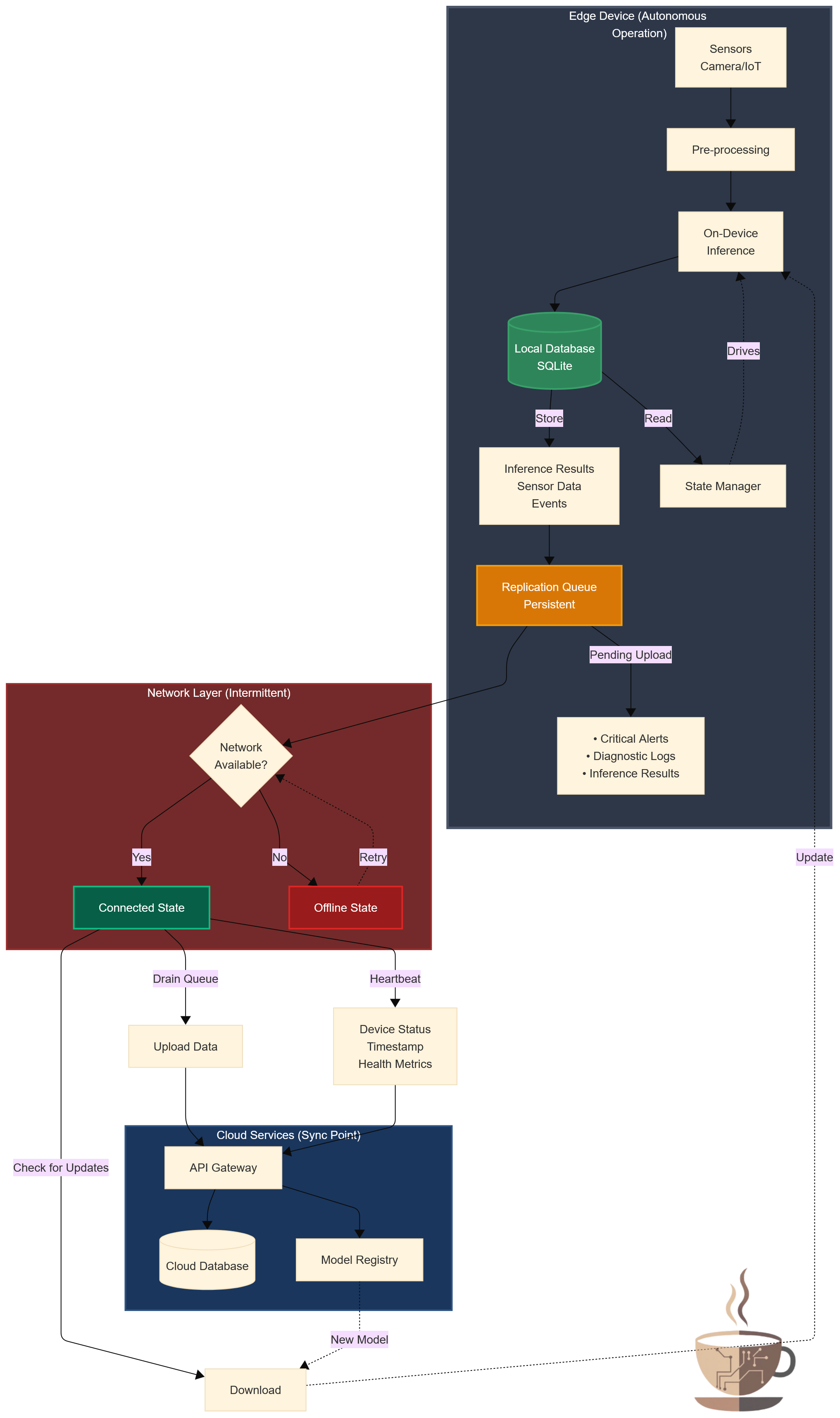
2. Offline-first: the default state of being
“Offline-first” is not a synonym for “caching.” Caching is a performance optimization that assumes the network is usually available and you’re just reducing latency. Offline-first is a philosophical stance that assumes the network is usually absent.
Core architectural components:
On-device data persistence: use a lightweight embedded database (SQLite is the canonical choice) to store:
Device state and configuration
Sensor readings with timestamps
Inference results and confidence scores
Events that need to be synchronized with the cloud
The device operates from this local state, and the cloud is eventually consistent with it, not the other way around.
Replication queues: any action that requires cloud coordination—uploading a critical alert, requesting a model update, logging a diagnostic event—goes into a persistent queue. When connectivity returns, the queue is drained. If connectivity drops mid-operation, the queue persists across reboots.
This requires careful design:
Operations must be idempotent (safe to retry)
Messages must have sequence numbers or timestamps for ordering
The queue must have a bounded size (what happens when it fills up?)
Heartbeats and state synchronization: when the network is available, the device’s job is not to depend on the cloud for real-time decisions. Its job is to synchronize state:
Send a heartbeat: “I’m alive, here’s my status.”
Upload queued data: “Here are the last 500 inference results.”
Check for updates: “Do you have a new model for me? New configuration?”
3. Quantization as an architectural contract
In most ML tutorials, quantization appears late in the story. You train a model in FP32. You evaluate it. Then, almost as an afterthought, you quantize it to INT8 to “make it smaller” and “run faster.” This framing is pedagogically convenient and architecturally backwards.
The systems reality: choosing hardware with dedicated INT8 acceleration is often an upfront decision driven by power and cost constraints. A neural accelerator that only supports INT8 might draw 500mW and cost $10. The equivalent FP32 accelerator might draw 3W and cost $50. For a battery-powered, cost-sensitive product, this decision is made before the data science team even starts collecting data.
This creates a contract: any model deployed to this hardware must be compatible with INT8 quantization and robust to the accuracy degradation it causes.
Consequences that flow through the entire system:
Quantization-Aware Training (QAT): you don’t train in FP32 and then quantize. You simulate quantization during training, allowing the model to learn weight distributions that are robust to the information loss.
Validation must test quantized performance: your holdout accuracy metrics in FP32 are irrelevant. The number that matters is the quantized model’s accuracy on the target hardware. If you don’t measure this, you don’t know if your system works.
Architecture choices are constrained: some operations quantize poorly. Large matrix multiplications with well-distributed weights quantize well. Softmax, layer normalization, and certain activation functions are problematic in INT8. Your model architect must avoid these or use hybrid precision (critical layers in FP16, most layers in INT8).
Conclusion
Edge deployment requires a fundamentally different approach than cloud-based ML.
Your objective is to build a device with sufficient intelligence to perform its function—detect defects, recognize objects, classify sounds—while operating within strict constraints on power, memory, connectivity, and latency. These constraints are not negotiable. They define what’s possible.
This demands a different mindset than training models in notebooks:
Power, memory, and latency are primary design constraints, not afterthoughts
Systems must degrade gracefully under stress, not fail catastrophically
Network connectivity is intermittent and unreliable by default
The entire system matters, not just the model
The cloud provides powerful abstractions. It makes compute feel infinite, memory abundant, and connectivity guaranteed. These abstractions have enabled enormous progress in ML.
The edge removes those abstractions. You work directly with physical constraints: finite energy, fixed memory, unreliable networks, real-time deadlines. This forces a shift from model optimization to systems engineering.
At the edge, the system is the product. The model is one component among many—sensors, power management, data pipelines, synchronization logic, failure handling. A perfect model in a fragile system is worthless. A good-enough model in a robust system ships and works.
The constraints are real. The physics is unforgiving. Design accordingly.